5 User Tutorial Section
The user Section contains the following sections: Basic Web Workflow Usage PEcAn Web Interface PEcAn from the Command Line
5.1 How PEcAn Works in a nutshell
PEcAn provides an interface to a variety of ecosystem models and attempts to standardize and automate the processes of model parameterization, execution, and analysis. First, you choose an ecosystem model, then the time and location of interest (a site), the plant community (or crop) that you are interested in simulating, and a source of atmospheric data from the BETY database (LeBauer et al, 2010). These are set in a “settings” file, commonly named pecan.xml which can be edited manually if desired. From here, PEcAn will take over and set up and execute the selected model using your settings. The key is that PEcAn uses models as-is, and all of the translation steps are done within PEcAn so no modifications are required of the model itself. Once the model is finished it will allow you to create graphs with the results of the simulation as well as download the results. It is also possible to see all past experiments and simulations.
There are two ways of using PEcAn, via the web interface and directly within R. Even for users familiar with R, using the web interface is a good place to start because it provides a high level overview of the PEcAn workflow. The quickest way to get started is to download the virtual machine or use an AWS instance.
5.2 PEcAn Demos
The following Tutorials assume you have installed PEcAn. If you have not, please consult the PEcAn Installation Section.
| Type | Title | Web Link | Source Rmd |
|---|---|---|---|
| Demo | Basic Run | html | Rmd |
| Demo | Uncertainty Analysis | html | Rmd |
| Demo | Output Analysis | html | Rmd |
| Demo | MCMC | html | Rmd |
| Demo | Parameter Assimilation | html | Rmd |
| Demo | State Assimilation | html | Rmd |
| Demo | Sensitivity | html | Rmd |
| Vignette | Allometries | html | Rmd |
| Vignette | MCMC | html | Rmd |
| Vignette | Meteorological Data | html | Rmd |
| Vignette | Meta-Analysis | html | Rmd |
| Vignette | Photosynthetic Response Curves | html | Rmd |
| Vignette | Priors | html | Rmd |
| Vignette | Leaf Spectra:PROSPECT inversion | html | Rmd |
5.3 Demo 01: Basic Run PEcAn
5.3.0.1 Objective
We will begin by exploring a set of web-based tools that are designed to run single-site model runs. A lot of the detail about what’s going on under the hood, and all the outputs that PEcAn produces, are left to Demo 2. This demo will also demonstrate how to use PEcAn outputs in additional analyses outside of PEcAn.
5.3.0.2 PEcAn URL
In the following demo, URL is the web address of a PEcAn server and will refer to one of the following:
- If you are doing a live demo with the PEcAn team, URL was provided
- If you are running the PEcAn virtual machine: URL = localhost:6480
- If you are running PEcAn using Amazon Web Services (AWS), URL is the Public IP
- If you are running PEcAn using Docker, URL is localhost:8000/pecan/ (trailing backslash is important!)
- If you followed instructions found in [Install PEcAn by hand], URL is your server’s IP
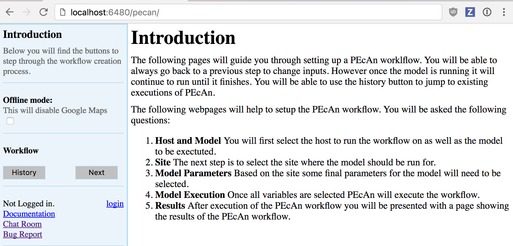
5.3.0.3 Start PEcAn:
- Enter URL in your web browser
- Click “Run Models”
- Click the ‘Next’ button to move to the “Site Selection” page.
5.3.0.4 Site Selection
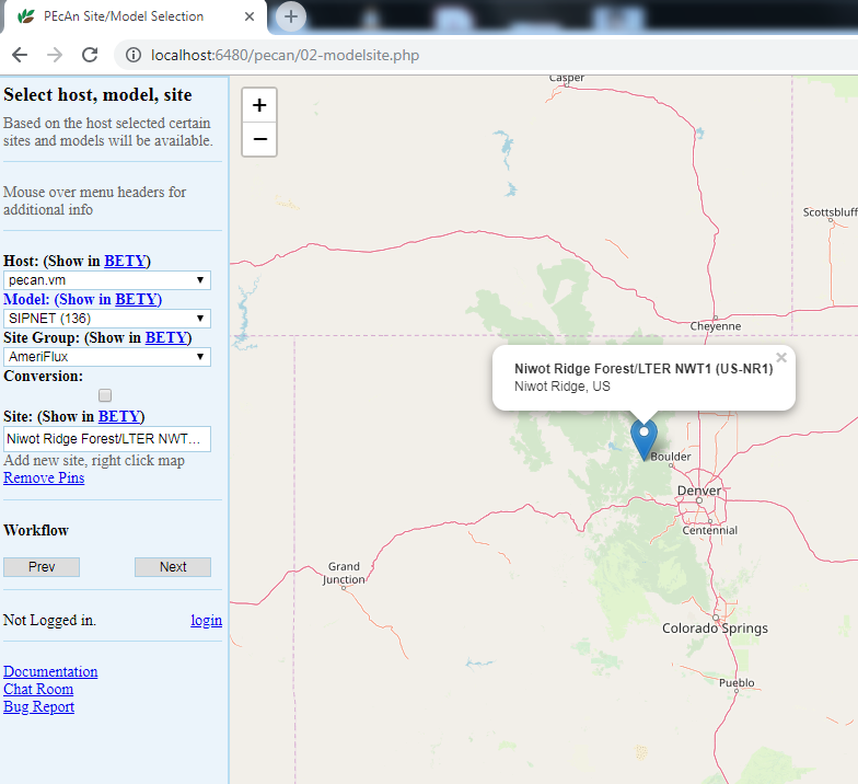
5.3.0.5 Host
Select the local machine “pecan”. Other options exist if you’ve read and followed instructions found in Remote execution with PEcAn.
5.3.0.6 Mode
Select SIPNET (r136) from the available models because it is quick & simple. Reference material can be found in [Models in PEcAn]
5.3.0.7 Site Group
To filter sites, you can select a specific group of sites. For this tutorial we will use Ameriflux.
5.3.0.8 Conversion:
Select the conversion check box, to show all sites that PEcAn is capable of generating model drivers for automatically. By default (unchecked), PEcAn only displays sites where model drivers already exist in the system database
5.3.0.9 Site:
For this tutorial, type US-NR1 in the search box to display the Niwot Ridge Ameriflux site (US-NR1), and then click on the pin icon. When you click on a site’s flag on the map, it will give you the name and location of the site and put that site in the “Site:” box on the left hand site, indicating your current selection.
Once you are finished with the above steps, click “Next”.
5.3.0.10 Run Specification
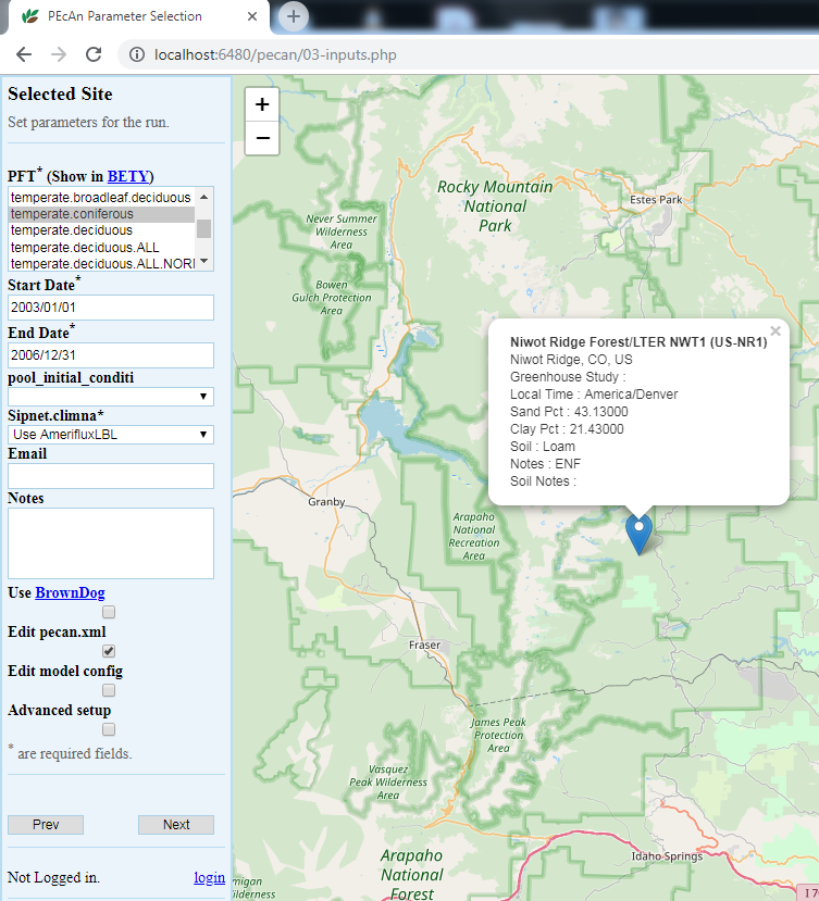
Next we will specify settings required to run the model. Be aware that the inputs required for any particular model may vary somewhat so there may be addition optional or required input selections available for other models.
5.3.0.11 PFT (Plant Functional Type):
Niwot Ridge is temperate coniferous. Available PFTs will vary by model and some models allow multiple competing PFTs to be selected. Also select soil to control the soil parameters
5.3.0.12 Start/End Date:
Select 2003/01/01 to 2006/12/31. In general, be careful to select dates for which there is available driver data.
5.3.0.13 Weather Data:
Select “Use AmerifluxLBL” from the Available Meteorological Drivers.
5.3.0.14 Optional Settings:
Leave all blank for demo run
- Email sends a message when the run is complete.
- Use Brown Dog will use the Brown Dog web services in order to do input file conversions. (Note: Required if you select Use NARR for Weather Data)
- Edit pecan.xml allows you to configure advanced settings via the PEcAn settings file
- Edit model config pauses the workflow after PEcAn has written all model specific settings but before the model runs are called and allows users to configure any additional settings internal to the model.
- Advanced Setup controls ensemble and sensitivity run settings discussed in Demo 2.
Finally, click “Next” to start the model run.
5.3.0.15 Data Use Policies
You will see a data policy statement if you selected a data source with a policy. Agreeing to the policy is required prior to starting the run.
5.3.0.16 If you get an error in your run
If you get an error in your run as part of a live demo or class activity, it is probably simplest to start over and try changing options and re-running (e.g. with a different site or PFT), as time does not permit detailed debugging. If the source of the error is not immediately obvious, you may want to take a look at the workflow.Rout to see the log of the PEcAn workflow or the logfile.txt to see the model execution output log and then refer to the Documentation or the Chat Room for help.
5.3.0.17 Model Run Workflow
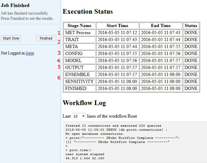
5.3.0.18 MET Process:
First, PEcAn will download meteorological data based on the type of the Weather Data you chose, and process it into the specific format for the chosen model
5.3.0.19 TRAIT / META:
PEcAn then estimates model parameters by performing a meta-analysis of the available trait data for a PFT. TRAIT will extract relevant trait data from the database. META performs a hierarchical Bayes meta-analysis of available trait data. The output of this analysis is a probability distribution for each model parameter. PEcAn selects the median value of this parameter as the default, but in Demo 2 we will see how PEcAn can use this parameter uncertainty to make probabilistic forecasts and assess model sensitivity and uncertainty. Errors at this stage usually indicate errors in the trait database or incorrectly specified PFTs (e.g. defining a variable twice).
5.3.0.20 CONFIG:
writes model-specific settings and parameter files
5.3.0.21 MODEL:
runs model.
5.3.0.22 OUTPUT:
All model outputs are converted to standard netCDF format
5.3.0.23 ENSEMBLE & SENSITIVITY:
If enabled post-process output for these analyses
If at any point a Stage Name has the Status “ERROR” please notify the PEcAn team member that is administering the demo or feel free to do any of the following:
- Refer to the PEcAn Documentation for documentation
- Post the end of your workflow log on our Gitter chat
- Post an issue on Github.
The entire PEcAn team welcomes any questions you may have!
If the Finished Stage has a Status of “DONE”, congratulations! If you got this far, you have managed to run an ecosystem model without ever touching a line of code! Now it’s time to look at the results click Finished.
FYI, adding a new model to PEcAn does not require modification of the model’s code, just the implementation of a wrapper function.
5.3.0.24 Output and Visualization
For now focus on graphs, we will explore all of PEcAn’s outputs in more detail in Demo 02.
5.3.0.25 Graphs
- Select a Year and Y-axis Variable, and then click ‘Plot run/year/variable’. Initially leave the X-axis as time.
- Within this figure the points indicate the daily mean for the variable while the envelope encompasses the diurnal variability (max and min).
- Variable names and units are based on a standard netCDF format.
- Try looking at a number of different output variables over different years.
- Try changing the X-axis to look at bivariate plots of how different output variables are related to one another. Be aware that PEcAn currently runs a moving min/mean/max through bivariate plots, just as it does with time series plots. In some cases this makes more sense than others.
5.3.0.26 Alternative Visualization: R Shiny
- Click on Open SHINY, which will open a new browser window. The shiny app will automatically access your run’s output files and allow you to visualize all output variables as a function of time.
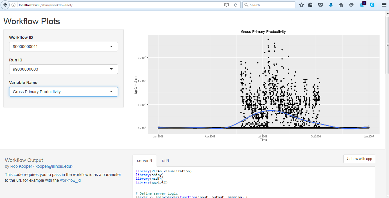
- Use the pull down menu under Variable Name to choose whichever output variable you wish to plot.
5.3.0.27 Model Run Archive
Return to the output window and Click on the HISTORY button. Click on any previous run in the “ID” column to go to the current state of that run’s execution – you can always return to old runs and runs in-progress this way. The run you just did should be the more recent entry in the table. For the next analysis, make note of the ID number from your run.
5.3.0.28 Next steps
5.3.0.28.1 Analyzing model output
Follow this tutorial, [Analyze Output] to learn how to open model output in R and compare to observed data
5.3.0.29 DEMO 02
Demo 02: Sensitivity and Uncertainty Analysis will show how to perform Ensemble & Sensitivity Analyses through the web interface and explore the PEcAn outputs in greater detail, including the trait meta-analysis
5.4 Demo 02: Sensitivity and Uncertainty Analysis
In Demo 2 we will be looking at how PEcAn can use information about parameter uncertainty to perform three automated analyses:
- Ensemble Analysis: Repeat numerous model runs, each sampling from the parameter uncertainty, to generate a probability distribution of model projections. Allows us to put a confidence interval on the model
- Sensitivity Analysis: Repeats numerous model runs to assess how changes in model parameters will affect model outputs. Allows us to identify which parameters the model is most sensitive to.
- Uncertainty Analysis: Combines information about model sensitivity with information about parameter uncertainty to determine the contribution of each model parameter to the uncertainty in model outputs. Allow us to identify which parameters are driving model uncertainty.
5.4.0.1 Run Specification
Return to the main menu for the PEcAn web interface: URL > Run Models
Repeat the steps for site selection and run specification from Demo 01, but also click on “Advanced setup”, then click Next.
By clicking Advanced setup, PEcAn will first show an Analysis Menu, where we are going to specify new settings.
For an ensemble analysis, increase the number of runs in the ensemble, in this case set Runs to 50. In practice you would want to use a larger ensemble size (100-5000) than we are using in the demo. The ensemble analysis samples parameters from their posterior distributions to propagate this uncertainty into the model output.
PEcAn’s sensitivity analysis holds all parameters at their median value and then varies each parameter one-at-a-time based on the quantiles of the posterior distribution. PEcAn also includes a handy shortcut, which is the default behavior for the web interface, that converts a specified standard deviation into its Normal quantile equivalent (e.g. 1 and -1 are converted to 0.157 and 0.841). In this example set Sensitivity to -2,-1,1,2 (the median value, 0, occurs by default).
We also can tell PEcAn which variable to run the sensitivity on. Here, set Variables to NEE, so we can compare against flux tower NEE observations.
Click Next
5.4.0.2 Additional Outputs:
The PEcAn workflow will take considerably longer to complete since we have just asked for over a hundred model runs. Once the runs are complete you will return to the output visualization page were there will be a few new outputs to explore, as well as outputs that were present earlier that we’ll explore in greater details:
5.4.0.3 Run ID:
While the sensitivity and ensemble analyses synthesize across runs, you can also select individual runs from the Run ID menu. You can use the Graphs menu to visualize each individual run, or open individual runs in Shiny
5.4.0.4 Inputs:
This menu shows the contents of /run which lets you look at and download:
- A summary file (README.txt) describing each run: location, run ID, model, dates, whether it was in the sensitivity or ensemble analysis, variables modifed, etc.
- The model-specific input files fed into the model
- The jobs.sh file used to submit the model run
5.4.0.5 Outputs:
This menu shows the contents of /out. A number of files generated by the underlying ecosystem model are archived and available for download. These include:
- Output files in the standardized netCDF ([year].nc) that can be downloaded for visualization and analysis (R, Matlab, ncview, panoply, etc)
- Raw model output in model-specific format (e.g. sipnet.out).
- Logfile.txt contains job.sh & model error, warning, and informational messages
5.4.0.6 PFTs:
This menu shows the contents of /pft. There is a wide array of outputs available that are related to the process of estimating the model parameters and running sensitivity/uncertainty analyses for a specific Plant Functional Type.
- TRAITS: The Rdata files trait.data.Rdata and madata.Rdata are, respectively, the available trait data extracted from the database that was used to estimate the model parameters and that same data cleaned and formatted for the statistical code. The list of variables that are queried is determined by what variables have priors associated with them in the definition of the PFTs. Priors are output into prior.distns.Rdata. Likewise, the list of species that are associated with a PFT determines what subset of data is extracted out of all data matching a given variable name. Demo 3 will demonstrate how a PFT can be created or modified. To look at these files in RStudio click on these files to load them into your workspace. You can further examine them in the Environment window or accessing them at the command line. For example, try typing
names(trait.data)as this will tell you what variables were extracted,names(trait.data$Amax)will tell you the names of the columns in the Amax table, andsummary(trait.data$Amax)will give you summary data about the Amax values. - META-ANALYSIS:
*.bug: The evaluation of the meta-analysis is done using a Bayesian statistical software package called JAGS that is called by the R code. For each trait, the R code will generate a [trait].model.bug file that is the JAGS code for the meta-analysis itself. This code is generated on the fly, with PEcAn adding or subtracting the site, treatment, and greenhouse terms depending upon the presence of these effects in the data itself. If the <random.effects> tag is set to FALSE then all random effects will be turned off even if there are multiple sites.meta-analysis.logcontains a number of diagnostics, including the summary statistics of the model, an assessment of whether the posterior is consistent with the prior, and the status of the Gelman-Brooks-Rubin convergence statistic (which is ideally 1.0 but should be less than 1.1).ma.summaryplots.*.pdfare collections of diagnostic plots produced in R after the above JAGS code is run that are useful in assessing the statistical model. Open up one of these pdfs to evaluate the shape of the posterior distributions (they should generally be unimodal), the convergence of the MCMC chains (all chains should be mixing well from the same distribution), and the autocorrelation of the samples (should be low).traits.mcmc.Rdatacontains the raw output from the statistical code. This includes samples from all of the parameters in the meta-analysis model, not just those that feed forward to the ecosystem, but also the variances, fixed effects, and random effects.post.distns.Rdatastores a simple tables of the posterior distributions for all model parameters in terms of the name of the distribution and its parameters.posteriors.pdfprovides graphics showing, for each model parameter, the prior distribution, the data, the smoothed histogram of the posterior distribution (labeled post), and the best-fit analytical approximation to that smoothed histogram (labeled approx). Open posteriors.pdf and compare the posteriors to the priors and data
- SENSITIVITY ANALYSIS
sensitivity.analysis.[RunID].[Variable].[StartYear].[EndYear].pdfshows the raw data points from univariate one-at-a-time analyses and spline fits through the points. Open this file to determine which parameters are most and least sensitive
- UNCERTAINTY ANALYSIS
variance.decomposition.[RunID].[Variable].[StartYear].[EndYear].pdf, contains three columns, the coefficient of variation (normalized posterior variance), the elasticity (normalized sensitivity), and the partial standard deviation of each model parameter. Open this file for BOTH the soil and conifer PFTS and answer the following questions:- The Variance Decomposition graph is sorted by the variable explaining the largest amount of variability in the model output (right hand column). From this graph identify the top-tier parameters that you would target for future constraint.
- A parameter can be important because it is highly sensitive, because it is highly uncertain, or both. Identify parameters in your output that meet each of these criteria. Additionally, identify parameters that are highly uncertain but unimportant (due to low sensitivity) and those that are highly sensitive but unimportant (due to low uncertainty).
- Parameter constraints could come from further literature synthesis, from direct measurement of the trait, or from data assimilation. Choose the parameter that you think provides the most efficient means of reducing model uncertainty and propose how you might best reduce uncertainty in this process. In making this choice remember that not all processes in models can be directly observed, and that the cost-per-sample for different measurements can vary tremendously (and thus the parameter you measure next is not always the one contributing the most to model variability). Also consider the role of parameter uncertainty versus model sensitivity in justifying your choice of what parameters to constrain.
5.4.0.7 PEcAn Files:
This menu shows the contents of the root workflow folder that are not in one of the folders indicated above. It mostly contains log files from the PEcAn workflow that are useful if the workflow generates an error, and as metadata & provenance (a detailed record of how data was generated).
STATUSgives a summary of the steps of the workflow, the time they took, and whether they were successfulpecan.*.xmlare PEcAn settings filesworkflow.Ris the workflow scriptworkflow.Routis the corresponding log filesamples.Rdatacontains the parameter values used in the runs. This file contains two data objects, sa.samples and ensemble.samples, that are the parameter values for the sensitivity analysis and ensemble runs respectivelysensitivity.output.[RunID].[Variable].[StartYear].[EndYear].Rdatacontains the object sensitivity.output which is the model outputs corresponding to the parameter values in sa.samples.- ENSEMBLE ANALYSIS
ensemble.Rdatacontains contains the object ensemble.output, which is the model predictions at the parameter values given in ensemble.samples.ensemble.analysis.[RunID].[Variable].[StarYear].[EndYear].pdfcontains the ensemble prediction as both a histogram and a boxplot.ensemble.ts.[RunID].[Variable].[StartYear].[EndYear].pdfcontains a time-series plot of the ensemble mean, median, and 95% CI
5.4.0.8 Global Sensitivity: Shiny
Navigate to URL/shiny/global-sensitivity.
This app uses the output from the ENSEMBLE runs to perform a global Monte Carlo sensitivity analysis. There are three modes controlled by Output type:
- Pairwise looks at the relationship between a specific parameter (X) and output (Y)
- All parameters looks at how all parameters affect a specific output (Y)
- All variables looks at how all outputs are affected by a specific parameter(X)
In all of these analyses, the app also fits a linear regression to these scatterplots and reports a number of summary statistics. Among these, the slope is an indicator of global sensitivity and the R2 is an indicator of the contribution to global uncertainty
5.4.0.9 Next Steps
The next set of tutorials will focus on the process of data assimilation and parameter estimation. The next two steps are in “.Rmd” files which can be viewed online.
5.4.0.10 Assimilation ‘by hand’
Explore how model error changes as a function of parameter value (i.e. data assimilation ‘by hand’)
5.4.0.11 MCMC Concepts
Explore Bayesian MCMC concepts using the photosynthesis module
5.4.0.12 More info about tools, analyses, and specific tasks…
Additional information about specific tasks (adding sites, models, data; software updates; etc.) and analyses (e.g. data assimilation) can be found in the PEcAn documentation
If you encounter a problem with PEcAn that’s not covered in the documentation, or if PEcAn is missing functionality you need, please search known bugs and issues, submit a bug report, or ask a question in our chat room. Additional questions can be directed to the project manager
5.5 Other Vignettes
5.5.1 Simple Model-Data Comparisons
5.5.1.2 Starting RStudio Server
Open RStudio Server in a new window at URL/rstudio
The username is carya and the password is illinois.
To open a new R script click File > New File > R Script
Use the Files browser on the lower right pane to find where your run(s) are located
All PEcAn outputs are stored in the output folder. Click on this to open it up.
Within the outputs folder, there will be one folder for each workflow execution. For example, click to open the folder PEcAn_99000000001 if that’s your workflow ID
A workflow folder will have a few log and settings files (e.g. pecan.xml) and the following subfolders
run     contains all the inputs for each run
out     contains all the outputs from each run
pft     contains the parameter information for each PFT
Within both the run and out folders there will be one folder for each unique model run, where the folder name is the run ID. Click to open the out folder. For our simple case we only did one run so there should be only one folder (e.g. 99000000001). Click to open this folder.
- Within this folder you will find, among other things, files of the format
.nc. Each of these files contains one year of model output in the standard PEcAn netCDF format. This is the model output that we will use to compare to data.
5.5.1.3 Read in settings From an XML file
## Read in the xml

settings<-PEcAn.settings::read.settings("~/output/PEcAn_99000000001/pecan.CONFIGS.xml")

## To read in the model output
runid<-as.character(read.table(paste(settings$outdir, "/run/","runs.txt", sep=""))[1,1]) # Note: if you are using an xml from a run with multiple ensembles this line will provide only the first run id
outdir<- paste(settings$outdir,"/out/",runid,sep= "")
start.year<-as.numeric(lubridate::year(settings$run$start.date))
end.year<-as.numeric(lubridate::year(settings$run$end.date))

site.id<-settings$run$site$id
File_path<-"~/output/dbfiles/AmerifluxLBL_site_0-772/AMF_US-NR1_BASE_HH_9-1.csv"

## Open up a connection to The Bety Database
bety <-dplyr::src_postgres(host = settings$database$bety$host, user = settings$database$bety$user, password = settings$database$bety$password, dbname = settings$database$bety$dbname)
5.5.1.4 Read in model output from specific variables
model_vars<-c("time", "NEE") #varibles being read
model <- PEcAn.utils::read.output(runid,outdir,start.year, end.year, model_vars,dataframe=TRUE)
The arguments to read.output are the run ID, the folder where the run is located, the start year, the end year, and the variables being read. The README file in the Input file dropdown menu of any successful run lists the run ID, the output folder, and the start and end year.
5.5.1.5 Compare model to flux observations
First load up the observations and take a look at the contents of the file
File_format<-PEcAn.DB::query.format.vars(bety = bety, format.id = 5000000002) #This matches the file with a premade "format" or a template that describes how the information in the file is organized

site<-PEcAn.DB::query.site(site.id,bety$con) #This tells PEcAn where the data comes from

observations<-PEcAn.benchmark::load_data(data.path = File_path, format= File_format, time.row = File_format$time.row,  site = site, start_year = start.year, end_year = end.year) #This will throw an error that not all of the units can be converted. That's ok, as the units of the varibles of interest (NEE) are being converted.
File_Path refers to where you stored your observational data. In this example the default file path is an Ameriflux dataset from Niwot Ridge.
File_format queries the database for the format your file is in. The defualt format ID “5000000002” is for csv files downloaded from the Ameriflux website. You could query for diffent kinds of formats that exist in bety or make your own.
Here 772 is the database site ID for Niwot Ridge Forest, which tells pecan where the data is from and what time zone to assign any time data read in.
Second apply a conservative u* filter to observations
Third align model output and observations
When we aligned the data, we got a dataframe with the variables we requested in a \(NEE.m\) and a \(NEE.o\) format. The \(.o\) is for observations, and the \(.m\) is for model. The posix column allows for easy plotting along a timeseries.
Fourth, plot model predictions vs. observations and compare this to a 1:1 line
## predicted vs observed plot
plot(aligned_dat$NEE.m, aligned_dat$NEE.o)
abline(0,1,col="red") ## intercept=0, slope=1Fifth, calculate the Root Mean Square Error (RMSE) between the model and the data
na.rm makes sure we don’t include missing or screened values in either time series.
Finally, plot time-series of both the model and data together
## plot aligned data
plot(aligned_dat$posix, aligned_dat$NEE.o, type="l")
lines(aligned_dat$posix,aligned_dat$NEE.m, col = "red")
Bonus How would you compare aggregated data?
Try RMSE against monthly NEE instead of half-hourly. In this case, first average the values up to monthly in the observations. Then, use align_data to match the monthly timestep in model output.
NOTE: Align_data uses two seperate alignment function, match_timestep and mean_over_larger_timestep. Match_timestep will use only that data that is present in both the model and the observation. This is helpful for sparse observations. Mean_over_larger_timestep aggregates the values over the largest timestep present. If you were to look at averaged monthly data, you would use mean_over_larger_timestep.
5.5.2 Data Assimilation Concepts
The goal of this tutorial is to help you gain some hands-on familiarity with some of the concepts, tools, and techniques involved in Bayesian Calibration. As a warm-up to more advanced approaches to model-data fusion involving full ecosystem models, this example will focus on fitting the Farquhar, von Caemmerer, and Berry (1980) photosynthesis model [FvCB model] to leaf-level photosynthetic data. This is a simple, nonlinear model consisting of 3 equations that models net carbon assimilation, \(A^{(m)}\), at the scale of an individual leaf as a function of light and CO2.
\[A_j = \frac{\alpha Q}{\sqrt{1+(\alpha^2 Q^2)/(Jmax^2)}} \frac{C_i- \Gamma}{4 C_i + 8 \Gamma}\]
\[A_c = V_{cmax} \frac{C_i - \Gamma}{C_i+ K_C (1+[O]/K_O) }\]
\[A^{(m)} = min(A_j,A_c) - r\]
The first equation \(A_j\) describes the RUBP-regeneration limited case. In this equation the first fraction is a nonrectangular hyperbola predicting \(J\), the electron transport rate, as a function of incident light \(Q\), quantum yield \(\alpha\), and the assymptotic saturation of \(J\) at high light \(J_{max}\). The second equation, \(A_c\), describes the Rubisco limited case. The third equation says that the overall net assimilation is determined by whichever of the two above cases is limiting, minus the leaf respiration rate, \(r\).
To keep things simple, as a Data Model (a.k.a. Likelihood or Cost Function) we’ll assume that the observed leaf-level assimilation \(A^{(o)}\) is Normally distributed around the model predictions with observation error \(\tau\).
\[A^{(o)} \sim N(A^{(m)},\tau)\]
To fit this model to data we’re going to rely on a piece of statistical software known as JAGS. The above model would be written in JAGS as:
model{

## Priors
  Jmax ~ dlnorm(4.7,2.7)             ## maximum electron transport rate prior
  alpha~dnorm(0.25,100)              ##quantum yield  (mol electrons/mole photon) prior
  vmax ~dlnorm(4.6,2.7)              ## maximum rubisco capacity prior

  r ~ dlnorm(0.75,1.56)              ## leaf respiration prior
  cp ~ dlnorm(1.9,2.7)               ## CO2 compensation point prior
  tau ~ dgamma(0.1,0.1)

  for(i in 1:n){

     ## electron transport limited
     Aj[i]<-(alpha*q[i]/(sqrt(1+(alpha*alpha*q[i]*q[i])/(Jmax*Jmax))))*(pi[i]-cp)/(4*pi[i]+8*cp)

     ## maximum rubisco limited without covariates
     Ac[i]<- vmax*(pi[i]-cp)/(pi[i]+Kc*(1+po/Ko))

     Am[i]<-min(Aj[i], Ac[i]) - r      ## predicted net photosynthesis
     Ao[i]~dnorm(Am[i],tau)            ## likelihood
     }

}
The first chunk of code defines the prior probability distributions. In Bayesian inference every unknown parameter that needs to be estimated is required to have a prior distribution. Priors are the expression of our belief about what values a parameter might take on prior to observing the data. They can arise from many sources of information (literature survey, meta-analysis, expert opinion, etc.) provided that they do not make use of the data that is being used to fit the model. In this particular case, the priors were defined by Feng and Dietze 2013. Most priors are lognormal or gamma, which were choosen because most of these parameters need to be positive.
After the priors is the Data Model, which in JAGS needs to be implemented as a loop over every observation. This is simply a codified version of the earlier equations.
Table 1: FvCB model parameters in the statistical code, their symbols in equations, and definitions
| Parameter | Symbol | Definition |
|---|---|---|
| alpha0 | \(\alpha\) | quantum yield (mol electrons/mole photon) |
| Jmax | \(J_{max}\) | maximum electron transport |
| cp | \(\Gamma\) | CO2 compensation point |
| vmax0 | \(V_{cmax}\) | maximum Rubisco capacity (a.k.a Vcmax) |
| r | \(R_d\) | leaf respiration |
| tau | \(\tau\) | residual precision |
| q | \(Q\) | PAR |
| pi | \(C_i\) | CO2 concentration |
5.5.2.1 Fitting the model
To begin with we’ll load up an example A-Ci and A-Q curve that was collected during the 2012 edition of the Flux Course at Niwot Ridge. The exact syntax below may be a bit confusing to those unaccustomed to R, but the essence is that the filenames line is looking up where the example data is stored in the PEcAn.photosynthesis package and the dat line is loading up two files (once A-Ci, the other A-Q) and concatanating them together.
library(PEcAn.photosynthesis)

### Load built in data
filenames <- system.file("extdata", paste0("flux-course-3",c("aci","aq")), package = "PEcAn.photosynthesis")
dat<-do.call("rbind", lapply(filenames, read_Licor))

## Simple plots
aci = as.character(dat$fname) == basename(filenames[1])
plot(dat$Ci[aci],dat$Photo[aci],main="ACi")
plot(dat$PARi[!aci],dat$Photo[!aci],main="AQ")
In PEcAn we’ve written a wrapper function, \(fitA\), around the statistical model discussed above, which has a number of other bells and whistles discussed in the PEcAn Photosynthesis Vignette. For today we’ll just use the most basic version, which takes as arguments the data and the number of MCMC iterations we want to run.
5.5.2.2 What’s going on
Bayesian numerical methods for model calibration are based on sampling parameter values from the posterior distribution. Fundamentally what’s returned is a matrix, with the number of iterations as rows and the number of parameters as columns, which are samples from the posterior distribution, from which we can approximate any quantity of interest (mean, median, variance, CI, etc.).
The following plots follow the trajectory of two correlated parameters, Jmax and alpha. In the first figure, arrows show the first 10 iterations. Internally JAGS is choosing between a variety of different Bayesian sampling methods (e.g. Metropolis-Hasting, Gibbs sampling, slice sampling, rejection sampling, etc) to draw a new value for each parameter conditional on the current value. After just 10 steps we don’t have a good picture of the overall posterior, but it should still be clear that the sampling is not a complete random walk.
params <- as.matrix(fit$params)
xrng = range(fit$params[,"alpha0"])
yrng = range(fit$params[,"Jmax0"])

n = 1:10
plot(params[n,"alpha0"],params[n,"Jmax0"],type='n',xlim=xrng,ylim=yrng)
arrows(params[n[-10],"alpha0"],params[n[-10],"Jmax0"],params[n[-1],"alpha0"],params[n[-1],"Jmax0"],length=0.125,lwd=1.1)
After 100 steps, we can see a cloud start to form, with occassional wanderings around the periphery.
After \(nrow(params)\) steps what we see is a point cloud of samples from the joint posterior distribution. When viewed sequentially, points are not independent, but we are interested in working with the overall distribution, where the order of samples is not important.
5.5.2.3 Evaluating the model output
A really important aspect of Bayesian inference is that the output is the joint posterior probability of all the parameters. This is very different from an optimization approach, which tries to find a single best parameter value. It is also different from estimating the independent posterior probabilities of each parameter – Bayesian posteriors frequently have strong correlation among parameters for reasons having to do both with model structure and the underlying data.
The model we’re fitting has six free parameters, and therefore the output matrix has 6 columns, of which we’ve only looked at two. Unfortunately it is impossible to visualize a 6 dimensional parameter space on a two dimensional screen, so a very common practice (for models with a small to medium number of parameters) is to look at all pairwise scatterplots. If parameters are uncorrelated we will typically see oval shaped clouds that are oriented in the same directions as the axes. For parameters with linear correlations those clouds will be along a diagonal. For parameters with nonlinear trade-offs the shapes of the parameter clouds can be more complex, such as the banana-shaped or triangular. For the FvCB model we see very few parameters that are uncorrelated or have simple linear correlations, a fact that we should keep in mind when interpreting individual parameters.
The three most common outputs that are performed on almost all Bayesian analyses are to look at the MCMC chains themselves, the marginal distributions of each parameter, and the overall summary statistics.
The ‘trace’ diagrams below show the history of individual parameters during the MCMC sampling. There are different color lines that represent the fact that JAGS ran the MCMC multiple times, with each run (i.e. each color) being refered to as a different \(chain\). It is common to run multiple chains in order to assess whether the model, started from different points, consistently converges on the same answer. The ideal trace plot looks like white noise with all chains in agreement.
The ‘density’ figures represent smoothed versions of the marginal distributions of each parameter. The tick marks on the x-axis are the actual samples. You will note that some posteriors will look approximately Normal, while others may be skewed or have clearly defined boundaries. On occassion there will even be posteriors that are multimodal. There is no assumption built into Bayesian statistics that the posteriors need be Normal, so as long as an MCMC has converged this diversity of shapes is valid. [note: the most common cause of multi-modal posteriors is a lack of convergence]
Finally, the summary table reports, for each parameter, a mean, standard deviation, two variants of standard error, and standard quantile estimates (95% CI, interquartile, and median). The standard deviation of the posterior is a good summary statistic about how uncertain we are about a parameter. The Naive SE is the traditonal \(\frac{SD}{\sqrt{n}}\), which is an estimate of the NUMERICAL accuracy in our estimate of the mean. As we run the MCMC longer (i.e. take more samples), we get an answer that is numerically more precise (SE converges to 0) but the uncertainty in the parameter (i.e. SD) stays the same because that’s determined by the sample size of the DATA not the length of the MCMC. Finally, the Time-series SE is a variant of the SE calculation that accounts for the autocorrelation in the MCMC samples. In practice is is therefore more appropriate to use this term to assess numerical accuracy.
plot(fit$params,auto.layout = FALSE)    ## MCMC diagnostic plots
summary(fit$params) ## parameter estimates
Assessing the convergence of the MCMC is first done visually, but more generally the use of statistical diagnostics to assess convergence is highly encouraged. There are a number of metrics in the literature, but the most common is the Gelman-Brooks-Rubin statistic, which compare the variance within each chain to the variance across chains. If the chains have converged then this quantity should be 1. Values less than 1.05 are typically considered sufficient by most statisticians, but these are just rules-of-thumb.
As with any modeling, whether statistical or process-based, another common diagnostic is a predicted vs observed plot. In a perfect model the data would fall along the 1:1 line. The deviations away from this line are the model residuals. If observations lie along a line other than the 1:1 this indicates that the model is biased in some way. This bias is often assessed by fitting a linear regression to the points, though two important things are noteworthy about this practice. First, the \(R^2\) and residual error of this regression are not the appropriate statistics to use to assess model performance (though you will frequently find them reported incorrectly in the literature). The correct \(R^2\) and residual error (a.k.a Root Mean Square Error, RMSE) are based on deviations from the 1:1 line, not the regression. The code below shows these two terms calculated by hand. The second thing to note about the regression line is that the standard regression F-test, which assesses deviations from 0, is not the test you are actually interested in, which is whether the line differs from 1:1. Therefore, while the test on the intercept is correct, as this value should be 0 in an unbiased model, the test statistic on the slope is typically of less interest (unless your question really is about whether the model is doing better than random). However, this form of bias can easily be assessed by looking to see if the CI for the slope overlaps with 1.
## predicted vs observed plot
par(mfrow=c(1,1))
mstats = summary(fit$predict)
pmean = mstats$statistics[grep("pmean",rownames(mstats$statistics)),1]
plot(pmean,dat$Photo,pch="+",xlab="Predicted A",ylab = "Observed A")
abline(0,1,col=2,lwd=2)
bias.fit = lm(dat$Photo~pmean)
abline(bias.fit,col=3,lty=2,lwd=2)
legend("topleft",legend=c("1:1","regression"),lwd=2,col=2:3,lty=1:2)
summary(bias.fit)
RMSE = sqrt(mean((pmean-dat$Photo)^2))
RMSE
R2 = 1-RMSE^2/var(dat$Photo)
R2
confint(bias.fit)
In the final set of plots we look at the actual A-Ci and A-Q curves themselves. Here we’ve added two interval estimates around the curves. The CI captures the uncertainty in the parameters and will asympotically shrink with more and more data. The PI (predictive interval) includes the parameter and residual error. If our fit is good then 95% PI should thus encompass at least 95% of the observations. That said, as with any statistical model we want to look for systematic deviations in the residuals from either the mean or the range of the PI.
Note: on the last figure you will get warnings about “No ACi” and “No AQ” which can be ignored. These are occuring because the file that had the ACi curve didn’t have an AQ curve, and the file that had the AQ curve didn’t have an ACi curve.
5.5.2.4 Additional information
There is a more detailed R Vignette on the use of the PEcAn photosynthesis module available in the PEcAn Repository.
5.5.2.5 Citations
Dietze, M.C. (2014). Gaps in knowledge and data driving uncertainty in models of photosynthesis. Photosynth. Res., 19, 3–14.
Farquhar, G., Caemmerer, S. & Berry, J.A. (1980). A biochemical model of photosynthetic CO2 assimilation in leaves of C3 species. Planta, 149, 78–90.
Feng, X. & Dietze, M.C. (2013). Scale dependence in the effects of leaf ecophysiological traits on photosynthesis: Bayesian parameterization of photosynthesis models. New Phytol., 200, 1132–1144.
5.5.3 Parameter Data Assimilation
5.5.3.1 Objectives
- Gain hands-on experience in using Bayesian MCMC techniques to calibrate a simple ecosystem model using parameter data assimilation (PDA)
- Set up and run a PDA in PEcAn using model emulation technique, assimilating NEE data from Niwot Ridge
- Examine outputs from a PDA for the SIPNET model and evaluation of the calibrated model against i) data used to constrain model, ii) additional data for the same site
5.5.3.2 Larger Context
Parameter data assimilation (PDA) occurs as one step in the larger process of model calibration, validation, and application. The goal of PDA is to update our estimates of the posterior distributions of the model parameters using data that correspond to model outputs. This differs from our previous use of PEcAn to constrain a simple model using data that map directly to the model parameters. Briefly, the recommended overall approach for model calibration and validation consists of the following steps:
- Assemble and process data sets required by the model as drivers
- Perform an initial test-run of the model as a basic sanity check
- Were there errors in drivers? (return to 1)
- Is the model in the same ballpark as the data?
- Construct priors for model parameters
- Collect/assemble the data that can be used to constrain model parameters and outputs
- Meta-analysis
- Sensitivity analysis (SA)
- Variance Decomposition (VD)
- Determine what parameters need further constraint
- Does this data exist in the literature? (repeat 4-8)
- Can I collect this data in the field? (repeat 4-8)
- Ensemble Analysis
- Is reality within the range of the uncertainty in the model?
- Evaluate/estimate uncertainties in the data
- Parameter Data Assimilation:
- Propose new parameter values
- Evaluate L(data | param) & prior(param)
- Accept or reject the proposed parameter values
- Repeat many times until a histogram of accepted parameter values approximates the true posterior distribution.
- Model evaluation [preferably ensemble based]
- Against data used to constrain model
- Against additional data for this site
- Same variable, different time
- Different variables
- Against data at a new site
- Do I need more data? Repeat 4-9 (direct data constraint) or 6-11 (parameter data assimilation).
- Application [preferably ensemble forecast or hindcast]
5.5.3.3 Connect to Rstudio
Today, we’re again going to work mostly in Rstudio, in order to easily edit advanced PEcAn settings and browse files. So if you haven’t already, connect now to the Rstudio server on your VM ([URL]/rstudio).
This tutorial assumes you have successfully completed an ensemble and a sensitivity analysis (Demo 2) before.
5.5.3.4 Defining variables
The following variables need to be set specific to the site being run and the workflow being run
workflow_id <- 99000000002  ## comes from the History table, your successful ensemble run's workflow ID

## from URL/bety/inputs.
##   Search by Ameriflux ID (e.g. US-NR1)
##   Find the "plain" site record (no CF or model name) that's on your server
##    (probably last in the list)
##   Click on the magnifying glass icon then look under "View Related Files"
datadir     <- "/home/carya/output/dbfiles/AmerifluxLBL_site_0-772/"

## where PEcAn is saving output (default OK on VM)
outdir      <- "/home/carya/output/"
5.5.3.5 Initial Ensemble Analysis
A good place to start when thinking about a new PDA analysis is to look at the current model fit to observed data. In fact, we want to compare data to a full ensemble prediction from the model. This is important because our current parameter distributions will be the priors for PDA. While the analysis will translate these priors into more optimal (in terms of producing model output that matches observations) and more confident (i.e. narrower) posterior distributions, these results are inherently constrained by the current parameter distributions. Thus, if reality falls far outside the prior ensemble confidence interval (which reflects the current uncertainty of all model parameters), data assimilation will not be able to fix this. In such cases, the prior parameter estimates must already be over-constrained, or there are structural errors in the model itself that need fixing. To begin, let’s load up some NEE observations so that we can plot them along with our ensemble predictions. In the code below the elements in bold may vary depending on site and your previous runs.
library(PEcAn.all)

# read settings
settings <- read.settings(file.path(outdir,paste0("PEcAn_",workflow_id),"pecan.CONFIGS.xml"))

# open up a DB connection
bety<-settings$database$bety
bety <-dplyr::src_postgres(host = bety$host, user = bety$user, password = bety$password, dbname = bety$dbname)

# Fill out the arguments needed by load_data function

# read file format information
format     <- PEcAn.DB::query.format.vars(bety = bety, format.id = 5000000002)
start_year <- lubridate::year(settings$run$start.date)
end_year   <- lubridate::year(settings$run$end.date)
vars.used.index <- which(format$vars$bety_name %in% c("NEE", "UST"))

obs <-PEcAn.benchmark::load_data(data.path = file.path(datadir, "AMF_US-NR1_BASE_HH_9-1.csv"),
                                 format = format, start_year = start_year,  end_year = end_year,
                                  site = settings$run$site,
                                  vars.used.index = vars.used.index,
                                  time.row = format$time.row)

obs$NEE[obs$UST<0.4] <- NA  ## U* filter
NEEo <- obs$NEE
Now let’s load up our ensemble outputs from the previous ensemble analysis (Demo 2) and plot our ensemble predictions against our NEE observations.
# load outputs, try not to delete prePDA ensemble output filename from your environment
prePDA_ensemble_output_file <- file.path(outdir,paste0("PEcAn_",workflow_id, "/ensemble.ts.", settings$ensemble$ensemble.id, ".NEE.2003.2006.Rdata"))
load(prePDA_ensemble_output_file)

# calculate CI
pre_pda_ens <- ensemble.ts[["NEE"]]
preCI <- apply(pre_pda_ens, 2, quantile, c(0.025, 0.5, 0.975), na.rm = TRUE)

# plot model ensemble
ymin <- min(min(c(preCI, NEEo), na.rm = TRUE))
ymax <- max(max(c(preCI, NEEo), na.rm = TRUE))
plot(preCI[2,], ylim = c(ymin, ymax), lwd = 2, xlab = "time", ylab = "NEE", main = "pre-PDA model ensemble vs data", type = "n")
prepoly <- 1:dim(preCI)[2]
polygon(c(prepoly, rev(prepoly)), c(preCI[3,], rev(preCI[1,])), col='khaki', border=NA)

# add data
points(NEEo, pch = ".", col= adjustcolor("purple",alpha.f=0.5))
legend("topright", legend=c("Data","Pre-PDA Model"), pch=c(15,15),
        col=c("purple","khaki"))
When interpreting your results it is important to remember the difference between a confidence interval, which just includes parameter uncertainties, and a predictive interval, which includes parameter and residual uncertainties. Your ensemble analysis plot illustrates the former—i.e., the confidence in the mean NEE. By contrast, the data reflect both changes in mean NEE, and random variability. As such, we can’t expect all the data to fall within the CI; in fact, if we had unlimited data to constrain mean NEE, the CI would collapse to a single line and none of the data would be contained! However, your plot will give you an idea of how much uncertainty there is in your model currently, and help to identify systematic errors like bias (values consistently too high or low) or poorly represented seasonal patterns.
5.5.3.6 Questions:
- Does your ensemble agree well with the data?
- If so, how much room for improvement is there, in terms of tightening the CI?
- If not, what are the greatest discrepancies?
- What are some of the problems (with model, data, and/or PEcAn) that might explain the data-model disparity you see?
5.5.3.7 Choosing Parameters
Beyond exploratory exercises, the first step of PDA analysis is to choose the model parameters you will target for optimization. PDA is computationally expensive (even when using an emulator), and the cost increases exponentially with the number of parameters targeted. The number you can handle in any given analysis completely depends on the complexity of the model and your available computational resources, but in practice it’s going to be rather small (~1–10) relative to the large number of parameters in a mechanistic ecosystem model (~10–100). Given this limitation, it is important to target parameters that can contribute substantially to improving model fit. If you recall, identifying those parameters was the goal of the uncertainty analysis you conducted previously, in the second PEcAn demo. Let’s revisit that analysis now. Open your variance decomposition graph from Demo 2 From this figure decide which variables you will target with PDA. As noted, an obvious criterion is that the parameter should be contributing a large amount of uncertainty to the current model, because otherwise it simply can’t change the model output much no matter how much you try to optimize it. But there are other considerations too. For example, if two parameters have similar or competing roles in the model, you may have trouble optimizing both simultaneously. In practice, there will likely be some guess-and-testing involved, though a good understanding of how the model works will help. It may also help to look at the shape of the Sensitivity responses and details of model fit to data (your ensemble analysis from the previous section). For the purposes of this demo, choose eight to ten parameters (in total, if you have more than one PFT) that contribute high uncertainty to model output and/or seem like good choices for some other rational reason.
5.5.3.8 Questions:
- Which parameters did you choose, and why?
5.5.3.9 Editing PEcAn settings
Now let’s add settings to tell PEcAn how to run the PDA with emulator, we will come to the details of model emulation later. Open up the pecan.CONFIGS.xml file you located previously, and choose File > Save as... from the menu to save a new copy as pecan.PDA.xml. Now add the block of XML listed below to the file, immediately after the <param.names><param> tags to identify the parameters you’ve chosen for PDA (it’s up to you to choose the number of parameters you want to constrain, then you can set the <n.knot> to be >= 10 per parameter you choose, e.g. 200 knots for 10 parameters). Here, you need to use PEcAn’s standard parameter names, which are generally not the same as what’s printed on your variance decomposition graph. To find your parameters look at the row names in the prior.distns.csv file for each PFT under the PFT pulldown menu. Insert the variable name (exactly, and case sensitive) into the <param> tags of the XML code below.
In addition, you may need to edit <inputs><file><path>, depending on the site and year you ran previously. The rest of the settings control options for the PDA analysis (how long to run, etc.), and also identify the data to be used for assimilation. For more details, see the assim.batch vignette on the PEcAn GitHub page (https://goo.gl/9hYVPQ).
<?xml version="1.0"?>    <-- These lines are already in there. Don't duplicate them,
<pecan>                  <-- just paste the <assim.batch> block below right after them.
  <assim.batch>
    <method>emulator</method>
    <n.knot>160</n.knot>                         <-- FILL IN
    <iter>25000</iter>
    <chain>3</chain>
    <param.names>
      <soil>
        <param>YOUR_PFT_1_PARAM_1</param>        <-- FILL IN
        <param>YOUR_PFT_1_PARAM_2</param>        <-- FILL IN
      </soil>
       <temperate.coniferous>
         <param>YOUR_PFT_2_PARAM_1</param>       <-- FILL IN
         <param>YOUR_PFT_2_PARAM_2</param>       <-- FILL IN
         <param>YOUR_PFT_2_PARAM_3</param>       <-- FILL IN
         <param>YOUR_PFT_2_PARAM_4</param>       <-- FILL IN
         <param>YOUR_PFT_2_PARAM_5</param>       <-- FILL IN
         <param>YOUR_PFT_2_PARAM_6</param>       <-- FILL IN
       </temperate.coniferous>
    </param.names>
    <jump>
        <adapt>100</adapt>
        <adj.min>0.1</adj.min>
        <ar.target>0.3</ar.target>
    </jump>
    <inputs>
     <file>
      <path>
         <path>/home/carya/output/dbfiles/AmerifluxLBL_site_0-772/AMF_US-NR1_BASE_HH_9-1.csv</path>
      </path>
      <format>5000000002</format>
      <input.id>1000011238</input.id>        <-- FILL IN, from BETY inputs table, this is *NOT* the workflow ID
      <likelihood>Laplace</likelihood>
      <variable.name>
        <variable.name>NEE</variable.name>
        <variable.name>UST</variable.name>
      </variable.name>
      <variable.id>297</variable.id>
     </file>
    </inputs>
  </assim.batch>
Once you’ve made and saved the changes to your XML, load the file and check that it contains the new settings:
settings <- read.settings(file.path(outdir,paste0("PEcAn_",workflow_id),"pecan.PDA.xml"))
settings$assim.batch
If the printed list contains everything you just added to pecan.PDA.xml, you’re ready to proceed.
5.5.3.10 Investigating PEcAn function pda.emulator (optional)
Before we run the data assimilation, let’s take a high-level look at the organization of the code. Use the Rstudio file browser to open up ~/pecan/modules/assim.batch/R/pda.emulator.R. This code works in much the same way as the pure statistical models that we learned about earlier in the week, except that the model being fit is a statistical model that emulates a complicated process-based computer simulation (i.e., an ecosystem model). We could have directly used the ecosystem model (indeed PEcAn’s other PDA functions perform MCMC by actually running the ecosystem model at each iteration, see pda.mcmc.R script as an example), however, this would require a lot more computational time than we have today. Instead here we will use a technique called model emulation. This technique allows us to run the model for a relatively smaller number of times with parameter values that have been carefully chosen to give a good coverage of parameter space. Then we can interpolate the likelihood calculated for each of those runs to get a surface that “emulates” the true likelihood and perform regular MCMC, except instead of actually running the model on every iteration to get a likelihood, this time we will just get an approximation from the likelihood emulator. The general algorithm of this method can be further expressed as:
- Propose initial parameter set sampling design
- Run full model for each parameter set
- Evaluate the likelihoods
- Construct emulator of multivariate likelihood surface
- Use emulator to estimate posterior parameter distributions
- (Optional) Refine emulator by proposing new design points, goto 2)
For now, we just want you to get a glimpse at the overall structure of the code, which is laid out in the comment headers in pda.emulator(). Most of the real work gets done by the functions this code calls, which are all located in the file ~/pecan/modules/assim.batch/R/pda.utils.R and the MCMC will be performed by the mcmc.GP() function in ~/pecan/modules/emulator/R/minimize.GP.R. To delve deeper into how the code works, take a look at these files when you have the time.
5.5.3.11 Running a demo PDA
Now we can go ahead and run a data assimilation MCMC with emulator. Since you’ve already loaded the settings containing your modified <assim.batch> XML block, all you need to do to start the PDA is run pda.emulator(settings). But, in the emulator workflow, there is a bit of a time consuming step where we calculate the effective sample size of the input data, and we have already done this step for you. You could load it up and pass it to the function explicitly in order to skip this step:
# load input data
load("/home/carya/pda/pda_externals.Rdata")
postPDA.settings <- pda.emulator(settings, external.data = inputs_w_neff)
After executing the code above, you will see print-outs to the console. The code begins with loading the prior values which in this case are the posterior distributions coming from your previous meta analysis. Then, normally, it loads the observational data and carries out necessary conversions and formatting to align it with model outputs, as we did separately above, but today it will skip this step as we are passing data externally. After this step, you will see a progress bar where the actual model is run n.knot times with the proposed parameter sets and then the outputs from these runs are read. Next, this model output is compared to the specified observational data, and the likelihood is calculated using the heteroskedastic Laplacian discussed previously. Once we calculate the likelihoods, we fit an emulator which interpolates the model output in parameter space between the points where the model has actually been run. Now we can put this emulator in the MCMC algorithm instead of the model itself. Within the MCMC loop the code proposes new parameter value from a multivariate normal jump distribution. The corresponding likelihood will be approximated by the emulator and the new parameter value is accepted or rejected based on its posterior probability relative to the current value.
5.5.3.12 Outputs from PEcAn’s Parameter Data Assimilation
When the PDA is finished, a number of outputs are automatically produced that are either the same as or similar to posterior outputs that we’ve seen before. These are located in the PEcAn_[workflow_id]/pft/* output directory and are identified by pda.[PFT]_[workflow_id] in the filenames:
- posteriors.pda.[PFT]*.pdf shows the posterior distributions resulting from your PDA
- trait.mcmc.pda.[PFT]*.Rdata contains all the parameter samples contained in the PDA posterior
- mcmc.pda.[PFT]*.Rdata is essentially the same thing in a different format
- mcmc.diagnostics.pda.[PFT]*.pdf shows trace plots and posterior densities for each assimilated parameter, as well as pairs plots showing all pairwise parameter correlations.
Together, these files allow you to evaluate whether a completed PDA analysis has converged and how the posterior distributions compare to the priors, and to use the posterior samples in further analyses, including additional PDA. If you haven’t done so already, take a look at all of the outputs described here.
5.5.3.13 Questions:
- Do the diagnostic figures indicate that your likelihood at least improved over the course of the analysis?
- Does the MCMC appear to have converged?
- Are the posterior distributions well resolved?
5.5.3.14 Post-PDA analyses
In addition to the outputs of the PDA itself, you may want to conduct ensemble and/or sensitivity analyses based on the posteriors of the data assimilation, in order to check progress towards improved model fit and/or changing sensitivity. For this, you need to generate new model runs based on parameters sampled from the updated (by PDA) posterior, which is a simple matter of rerunning several steps of the PEcAn workflow.
The PDA you ran has automatically produced an updated XML file (pecan.pda***.xml) that includes the posterior id to be used in the next round of runs. Locate this file in your run directory and load the file for the post-pda ensemble/sensitivity analysis (if you already have the settings list in your working environment you don’t need to re-read the settings):
 # read post-PDA settings if you don't have them in your wotking environment
 # replace the *** with the ensemble id given by the workflow
 # postPDA.settings <- read.settings(file.path(outdir,paste0("PEcAn_", workflow_id),"pecan.pda***.xml"))

 # Call model specific write.configs
  postPDA.settings <- run.write.configs(postPDA.settings,
                          write=postPDA.settings$database$bety$write,
                          ens.sample.method=postPDA.settings$ensemble$method)

 # Let's save the settings with the new ensemble id
  PEcAn.settings::write.settings(settings, outputfile=paste0('pecan.pda', postPDA.settings$assim.batch$ensemble.id,'.xml'))

 # Start ecosystem model runs, this one takes awhile...
  PEcAn.remote::start.model.runs(postPDA.settings, postPDA.settings$database$bety$write)

 # Get results of model runs
  get.results(postPDA.settings)

 # Repeat ensemble analysis with PDA-constrained params
 run.ensemble.analysis(postPDA.settings, TRUE)

 # let's re-load the pre-PDA ensemble outputs
 load(prePDA_ensemble_output_file)
 pre_pda_ens <- ensemble.ts[["NEE"]]

 # nowload the post-PDA ensemble outputs
 postPDA_ensemble_output_file <- file.path(outdir,paste0("PEcAn_", workflow_id, "/ensemble.ts.", postPDA.settings$ensemble$ensemble.id, ".NEE.2003.2006.Rdata"))
 load(postPDA_ensemble_output_file)
 post_pda_ens <- ensemble.ts[["NEE"]]

 # try changing the window value for daily, weekly, monthly smoothing later
 # see if this changes your model-data agreement, why?
 window <- 1 # no smoothing
 pre_pda <- t(apply(pre_pda_ens, 1, function(x) {
        tapply(x, rep(1:(length(x)/window + 1), each = window)[1:length(x)],
               mean, na.rm = TRUE)}))
 post_pda <- t(apply(post_pda_ens, 1, function(x) {
        tapply(x, rep(1:(length(x)/window + 1), each = window)[1:length(x)],
               mean, na.rm = TRUE)}))
 fobs <- tapply(NEEo, rep(1:(length(NEEo) / window + 1),
                          each = window)[1:length(NEEo)], mean, na.rm = TRUE)


 # save the comparison plots to pdf
 pdf(file.path(outdir,paste0("PEcAn_",workflow_id),"model.data.comparison.pdf"), onefile=T,
     paper='A4r', height=15, width=20)

 # now plot the pre-PDA ensemble similar to the way we did before
 preCI <- apply(pre_pda, 2, quantile, c(0.025, 0.5, 0.975), na.rm = TRUE)
 ymin <- min(min(c(preCI, fobs), na.rm = TRUE))
 ymax <- max(max(c(preCI, fobs), na.rm = TRUE))
 plot(pre_pda[1,], ylim = c(ymin, ymax), lwd = 2, xlab = "time", ylab = "NEE", main = "pre-PDA vs post-PDA", type = "n")
 prepoly <- 1:dim(preCI)[2]
 polygon(c(prepoly, rev(prepoly)),c(preCI[3,], rev(preCI[1,])),col='khaki',border=NA)

 # plot the post-PDA ensemble
 postCI <- apply(post_pda, 2, quantile, c(0.025, 0.5, 0.975), na.rm = TRUE)
 postpoly <- 1:dim(postCI)[2]
 polygon(c(postpoly, rev(postpoly)),c(postCI[3,], rev(postCI[1,])),col='lightblue',border=NA)

 # finally let's add the data and see how we did
 points(fobs, pch = ".", col= adjustcolor("purple",alpha.f=0.7))
 legend("topright", legend=c("Data","Pre-PDA Model", "Post-PDA Model"), pch=c(15,15,15),
        col=c("purple","khaki","lightblue"))

 dev.off()


 # Repeat variance decomposition to see how constraints have changed
 run.sensitivity.analysis(postPDA.settings)
Now you can check the new figures produced by your analyses under PEcAn_[workflow_id]/pft/*/variance.decomposition.*.pdf and PEcAn_[workflow_id]/pft/*/sensitivity.analysis.*.pdf, and compare them to the previous ones. Also, take a look at the comparison of model outputs to data when we run SIPNET with pre- and post-PDA parameter (mean) values under PEcAn_[workflow_id]/model.data.comparison.pdf.
5.5.3.15 Questions:
- Looking at the ensemble analysis outputs in order (i.e., in order of increasing ID in the filenames), qualitatively how did the model fit to data change over the course of the analysis?
- Based on the final ensemble analysis, what are the major remaining discrepancies between model and data?
- Can you think of the processes / parameters that are likely contributing to the differences?
- What would be your next steps towards evaluating or improving model performance?
5.5.4 State-Variable Data Assimilation
5.5.4.1 Objectives:
- Assimilate tree ring estimated NPP & inventory AGB within the SIPNET model in order to:
- Reconcile data and model NPP & AGB estimates
- Constrain inferences about other ecosystem responses.
5.5.4.2 Overview:
- Initial Run
- Settings
- Load and match plot and increment data
- Estimate tree-level data uncertainties
- Estimate allometric relationships
- Estimate stand-level NPP
- Sample initial conditions and parameters
- Run Ensemble Kalman Filter
5.5.4.3 Initial Run
Perform a site-level SIPNET run using the following settings
- Site = UNDERC
- Start = 01/01/1979
- End = 12/31/2015
- Met = NARR
- Check Brown Dog
- When the run is complete, open the pecan.xml and cut-and-paste the outdir for later use
5.5.4.4 Settings:
Open the PEcAn RStudio environment back up.
Set your working directory to the outdir from above
setwd(outdir)and shift the file browser to that location (Files > More > Go To Working Directory)Open up the latest settings file
pecan.CONFIG.xml.At the top of the file add the following tags to set the ensemble size
   <state.data.assimilation>
   <n.ensemble>35</n.ensemble>
   <process.variance>FALSE</process.variance>
   <sample.parameters>TRUE</sample.parameters>
   <data>
    <format_id>1000000040</format_id>
    <input.id>1000013298</input.id>
  </data>
   <state.variables>
   <variable>
   <variable.name>NPP</variable.name>
   <unit>MgC/ha/yr</unit>
        <min_value>-9999</min_value>
        <max_value>9999</max_value>
   </variable>
   <variable>
   <variable.name>AbvGrndWood</variable.name>
       <unit>KgC/m^2</unit>
       <min_value>0</min_value>
       <max_value>9999</max_value>
   </variable>
   <variable>
   <variable.name>TotSoilCarb</variable.name>
      <unit>KgC/m^2</unit>
      <min_value>0</min_value>
      <max_value>9999</max_value>
   </variable>
   <variable>
   <variable.name>LeafC</variable.name>
         <unit>m^2/m^2</unit>
         <min_value>0</min_value>
         <max_value>9999</max_value>
   </variable>
   <variable>
   <variable.name>SoilMoistFrac</variable.name>
         <unit></unit>
         <min_value>0</min_value>
         <max_value>9999</max_value>
   </variable>
   <variable>
   <variable.name>SWE</variable.name>
         <unit>cm</unit>
         <min_value>0</min_value>
         <max_value>9999</max_value>
   </variable>
   <variable>
   <variable.name>Litter</variable.name>
         <unit>gC/m^2</unit>
         <min_value>0</min_value>
         <max_value>9999</max_value>
   </variable>
   </state.variables>
   <forecast.time.step>year</forecast.time.step>
  <start.date>1980/01/01</start.date>
  <end.date>2015/12/31</end.date>
  </state.data.assimilation>
Delete the `
<pfts>block from the settingsIn the PEcAn History, go to your PDA run and open
pecan.pda[UNIQUEID].xml(the one PEcAn saved for you AFTER you finished the PDA)Cut-and-paste the PDA
<pfts>block into the SDA settings fileSave the file as
pecan.SDA.xml
5.5.4.5 Loading data
- If you have not done so already, clone (new) or pull (update) the PalEON Camp2016 repository
- Open a shell under Tools > Shell
- `
cdto go to your home directory - To clone:
git clone git@github.com:PalEON-Project/Camp2016.git To pull:
cd Camp2016; git pull https://github.com/PalEON-Project/Camp2016.git masterOpen the tree-ring data assimilation workflow under Home > pecan > scripts > workflow.treering.R
Run the script from the start up through the LOAD DATA section
5.5.4.6 Estimating tree-level data uncertainties
One thing that is critical for data assimilation, whether it is being used to estimate parameters or state variables, is the careful consideration and treatment of the uncertainties in the data itself. For this analysis we will be using a combination of forest plot and tree ring data in order to estimate stand-level productivity. The basic idea is that we will be using the plot-sample of measured DBHs as an estimate of the size structure of the forest, and will use the annual growth increments to project that forest backward in time. Tree biomass is estimated using empirical allometric equations relating DBH to aboveground biomass. There are a number of sources of uncertainty in this approach, and before moving you are encouraged to think about and write down a few:
Today we will use a statistical model based on the model developed by Clark et al 2007 that partitions out a number of sources of variability and uncertainty in tree ring and plot data (Fig 1). This model is a Bayesian statespace model that treats the true diameters (D) and increments (X) as latent variables that are connected through a fairly simple mixed effects process model
\[D_{ij,t+1} = D_{ij,t} + \mu + \alpha_{i} + \alpha_t + \epsilon_{ij,t}\]
where i = individual, j = plot, t = time (year). Each of these terms are represented at normal distributions, where \(\mu\) is a fixed effect (overall mean growth rate) and individual and year are random effects
\[\mu \sim N(0.5,0.5)\] \[\alpha_{i} \sim N(0,\tau_{i})\] \[\alpha_{t} \sim N(0,\tau_{t})\] \[\epsilon_{ij,t} \sim N(0,\tau_{e})\]
The connection between the true (latent) variable and the observations is also represented as normal with these variances representing measurement error:
\[D_{ij,t}^O \sim N( D_{ij,t},\tau_D)\] \[X_{ij,t}^O \sim N( X_{ij,t},\tau_r)\]
Finally, there are five gamma priors on the precisions, one for the residual process error (\(\tau_{e}\)), two for the random effects on individual (\(\tau_{i}\)) and time (\(\tau_t\)), and two measurement errors or DBH (\(\tau_D\)) and tree rings (\(\tau_r\))
\[\tau_{e} \sim Gamma(a_e,r_e)\] \[\tau_{i} \sim Gamma(a_i,r_i)\] \[\tau_{t} \sim Gamma(a_t,r_t)\] \[\tau_{D} \sim Gamma(a_D,r_D)\] \[\tau_{r} \sim Gamma(a_r,r_r)\]
This model is encapsulated in the PEcAn function:
where the first argument is the combined data set formatted for JAGS and the second is the number of MCMC interations. The model itself is written for JAGS and is embedded in the function. Running the above InventoryGrowthFusion will run a full MCMC algorithm, so it does take a while to run. The code returns the results as an mcmc.list object, and the next line in the script saves this to the outputs directory We then call the function InventoryGrowthFusionDiagnostics to print out a set of MCMC diagnostics and example time-series for growth and DBH.
5.5.4.7 Allometric equations
Aboveground NPP is estimated as the increment in annual total aboveground biomass. This estimate is imperfect, but not unreasonable for demonstration purposes. As mentioned above, we will take an allometric approach of scaling from diameter to biomass: Biomass = b0 * DBH b1 We will generate the allometric equation on a PFT level using another Bayesian model that synthesizes across a database of species-level allometric equations (Jenkins et al 2004). This model has two steps within the overall MCMC loop. First it simulates data from each equation, including both parameter and residual uncertainties, and then it updated the parameters of a single allometric relationship across all observations. The code also fits a second model, which includes a random site effect, but for simplicity we will not be using output from this version. Prior to running the model we have to first query the species codes for our pfts. Next we pass this PFT list to the model, AllomAve, which saves the results to the output directory in addition to returning a summary of the parameters and covariances.
5.5.4.8 Estimate stand-level NPP
If we have no uncertainty in our data or allometric equations, we could estimate the stand aboveground biomass (AGB) for every year by summing over the biomass of all the trees in the plot and then divide by the plot area. We would then estimate NPP by the difference in AGB between years. One approach to propagating uncertainties into NPP would be to transform the distribution of DBH for each individual tree and year into a distribution for biomass, then sum over those distributions to get a distribution for AGB and then subtract the distributions to get the distributions of NPP. However, if we do this we will greatly overestimate the uncertainty in NPP because we ignore the fact that our increment data has much lower uncertainty than our diameter data. In essence, if we take a random draw from a distribution of AGB in year and it comes back above average, the AGB is much more likely to also be above average the following year than if we were to do an independent draw from that distribution. Accounting for this covariance requires a fairly simple change in our approach and takes advantage of the nature of the MCMC output. The basic idea is that we are going to take a random draw from the full individual x year diameter matrix, as well as a random draw of allometric parameters, and perform the ‘zero-error’ calculation approach described above. We will then create a distribution of all the NPP estimates that comes out of repeated draws for the full diameter matrix. This approach is encapsulated in the function plot2AGB. The argument unit.conv is a factor that combines both the area of the plot and the unit conversion from tree biomass (kg/tree) to stand AGB (Mg/ha). There are two outputs from plot2AGB: a pdf depicting estimated NPP and AGB (mean and 95% CI) time series, with each page being a plot; and plot2AGB.Rdata, a binary record of the function output that is read into the data assimilation code. The latter is also returned from the fuction and assigned to the variable “state”. Finally, we calculate the mean and standard deviation of NPP and save this as obs.
5.5.4.9 Build Initial Conditions
The function sample.IC.SIPNET uses the AGB estimate from the previous function in order to initialize the data assimilation routine. Specifically it samples n.ensemble values from the first time step of the AGB estimate. Embedded in this function are also a number of prior distributions for other state variables, which are also samples in order to create a full set of initial conditions for SIPNET.
5.5.4.10 Load Priors
The function sample.parameters samples values from the most recent posterior parameter distributions. You can also specify a specific set of parameters so sample from by specifying the argument <prior> within <assim.sequential> as the posterior.id you want to use. This is useful to know if you want to go back and run with the Meta-analysis posteriors, or if you end up rerunning the meta-analysis and need to go back and specify the parameter data assimilation posteriors instead of the most recent.
5.5.4.11 Ensemble Kalman Filter
The function sda.enkf will run SIPNET in Ensemble Kalman Filter mode. The output of this function will be all the of run outputs, a PDF of diagnostics, and an Rdata object that includes three lists:
- FORECAST will be the ensemble forecasts for each year
- ANALYSIS will be the updated ensemble sample given the NPP observations
- enkf.params contains the prior and posterior mean vector and covariance matrix for each time step.
If you look within this function you will find that much of the format is similar to the pda.mcmc function, but in general is much simpler. The function begins by setting parameters, opening a database connection, and generating workflow and ensemble ID’s. Next we split the SIPNET clim meteorology file up into individual annual files since we will be running SIPNET for a year at a time between updates. Next we perform an initial set of runs starting from the initial states and parameters we described above. In doing so we create the run and output directories, the README file, and the runs.txt file that is read by start.model.runs. Worth noting is that the README and runs.txt don’t need to be updated within the forecast loop. Given this initial run we then enter the forecast loop. Within this loop over years we perform four basic steps. First, we read the output from the latest runs. Second, we calculate the updated posterior state estimates based on the model ensemble prior and observation likelihood. Third, we resample the state estimates based on these posterior parameters. Finally, we start a new set of runs based on this sample. The sda.enfk function then ends by saving the outputs and generating some diagnostic figures. The first set of these shows the data, forecast, analysis. The second set shows pairs plots of the covariance structure for the Forecast and Analysis steps. The final set shows the time-series plots for the Analysis of the over state variables produced by SIPNET.
5.5.4.12 Finishing up
The final bit of code in the script will register the workflow as complete in the database. After this is run you should be able to find all of the runs, and all of the outputs generated above, from within the PEcAn webpages.
5.5.5 PEcAn: Testing the Sensitivity Analysis Against Observations"
5.5.5.2 Flux Measurements and Modeling Course, Tutorial Part 2
This tutorial assumes you have successfully completed the Demo01, Demo02 and the modelVSdata tutorial.
5.5.5.3 Introduction
Now that you have successfully run PEcAn through the web interface and have learned how to do a simple comparison of flux tower observations to model output, let’s start looking at how data assimilation and parameter estimation would work with an ecosystem model.
Before we start a full data assimilation exercise, let’s try something simple – single parameter selection by hand.
- Open http://localhost:3280/rstudio or http://localhost:6480/rstudio or the Amazon URL/rstudio if running on the cloud.
In Demo02, you have ran a sensitivity analysis of SIPNET model runs at Niwot Ridge sampling across quantiles of a parameter prior, while holding all others to the median value. The pecan.xml file told PEcAn to run an sensitivity analysis, which simply meant SIPNET was run multiple times with the same driver, but varying parameter values one at a time (while holding all others to their median), and the parameter range also specified in the pecan.xml file (as quantiles, which were then sampled against the BETY database of observed variation in the parameter for species within the specific plant functional type).
Let’s try to compare Ameriflux NEE to SIPNET NEE across all these runs to make a plot of parameter vs. goodness-of-fit. We’ll start with root mean square error (RMSE), but then discuss some other tests, too.
5.5.5.4 A. Read in settings object from a run xml
Open up a connection to the bety database and create a settings object from your xml, just like in the modelVSdata tutorial.
settings<-PEcAn.settings::read.settings("~/output/PEcAn_99000000002/pecan.CONFIGS.xml")

bety<-settings$database$bety
bety <-dplyr::src_postgres(host = bety$host, user = bety$user, password = bety$password, dbname = bety$dbname)
We read in the pecan.CONFIG.xml instead of the pecan.xml because the pecan.CONFIG.xml has already incorperated some of the information from the database we would have to query again if we used the pecan.xml.
runid<-as.character(read.table(paste(settings$outdir, "/run/","runs.txt", sep=""))[1,1]) # Note: if you are using an xml from a run with multiple ensembles this line will provide only the first run id
outdir<- paste(settings$outdir,"/out/",runid,sep= "")
start.year<-as.numeric(lubridate::year(settings$run$start.date))
end.year<-as.numeric(lubridate::year(settings$run$end.date))

site.id<-settings$run$site$id
Back to the files pane, within the run/ folder, find a folder called pft/ and within that a folder with the pft name (such as temprature.coniferous). Within that is a PDF file that starts sensitivity.analysis. In Rstudio, just click on the PDF to view it. You discussed this PDF last tutorial, through the web interface. Here, we see how the model NEE in SIPNET changes with each parameter.
Let’s read that sensitivity output. Navigate back up (..) to the ~/output/RUNDIR/ folder. Find a series of files that end in “.RData”. These files contain the R variables used to make these plots. In particular, there is sensitivity.output..RData which contains the annual NEE as a function of each parameter quantile. Click on it to load a variable into your environment. There is sensitivity.results..RData which contains plotting functions and variance decomposition output, which we don’t need in this tutorial. And finally, there is **sensitivity.samples.*.RData** which contains the actual parameter values and the RunIDs associated with each sensitivity run.
Click on sensitivity.samples..RData* to load it into your environment, or run the {r}load() script below. You should see a set of five new variables (pft.names, trait.names, sa.ensemble.id, sa.run.ids, sa.samples).
Let’s extract a parameter and it’s sensitivity NEE output from the list sa.samples, which is organized by PFT, and then by parameter. First, let’s look at a list of PFTs and parameters available:
load(paste(settings$outdir,"/sensitivity.samples.", settings$sensitivity.analysis$ensemble.id,".Rdata", sep=""))

names(sa.samples)
names(sa.samples$temperate.coniferous)
Now to see the actual parameter values used by the runs, just pick a parameter and type:
Let’s store that value for future use:
Now, to see the annual NEE output from the model for a particular PFT and parameter range, try
load(paste(settings$outdir,paste("/sensitivity.output", settings$sensitivity.analysis$ensemble.id,settings$sensitivity.analysis$variable,start.year,end.year,"Rdata", sep="."), sep=""))

sensitivity.output$temperate.coniferous$psnTOpt
You could even plot the two:
What do you notice?
Let’s try to read the output from a single run id as you did in the earlier tutorial.
5.5.5.5 B. Now let’s bring in the actual observations
Recall reading Ameriflux NEE in the modelVSdata tutorial.
File_path<-"~/output/dbfiles/AmerifluxLBL_site_0-772/AMF_US-NR1_BASE_HH_9-1.csv"

File_format<-PEcAn.DB::query.format.vars(bety = bety, format.id = 5000000002) #This matches the file with a premade "format" or a template that describes how the information in the file is organized
site<-PEcAn.DB::query.site(site.id = site.id,bety$con)

obs<-PEcAn.benchmark::load_data(data.path = File_path, format= File_format, time.row = File_format$time.row,  site = site, start_year = start.year, end_year = end.year)

obs$NEE[obs$UST<0.2]<-NA #Apply a U* filter

plottable<-align_data(model.calc = arun, obvs.calc = obs, align_method = "match_timestep", var= "NEE")
head(plottable)
5.5.5.6 C. Finally, we can finally compare model to data
In the modelVSdata, you also compared NEE to the ensemble model run. Here we will do the same except we include each sensitivity run.
And remember the formula for RMSE:
All we need to do to go beyond this is to make a loop that reads in each sensitivity run NEE based on runids, calculates RMSE against the observations, and stores it in an array, by combining the steps above in a for loop. Make sure you change the directory names and year to your specific run.
rmses <- rep(0,length(runids))
for(r in 1:length(runids)){
arun <- read.output(runids[r],paste(settings$outdir, "out", runids[r], sep="/"),2004,2004,"NEE", dataframe= TRUE)
plottable<-align_data(model.calc = arun, obvs.calc = obs, align_method = "match_timestep", var= "NEE")
rmses[r] <- sqrt(mean((plottable$NEE.o-plottable$NEE.m)^2,na.rm = TRUE))
}

rmses
Let’s plot that array
Can you identify a minimum (if there is one)? If so, is there any reason to believe this is the “best” parameter? Why or why not? Think about all the other parameters.
Now that you have the hang of it, here are a few more things to try:
- Try a different error functions, given actual NEE uncertainty. You learned earlier that uncertainty in half-hourly observed NEE is not Gaussian. This makes RMSE not the correct measure for goodness-of-fit. Go to ~/pecan/modules/uncertainty/R, open flux_uncertainty.R, and click on the source button in the program editing pane.
Alternatively, you can source the function from the console using:
Then you can run:
The figure shows you uncertainty (err) as a function of NEE magnitude (mag). How might you use this information to change the RMSE calculation?
Try a few other parameters. Repeat the above steps but with a different parameter. You might want to select one from the sensitivity PDF that has a large sensitivity or from the variance decomposition that is also poorly constrained.
5.6 Advanced User Guide
5.6.1 Submitting Workflow from Command Line
This is how you can submit a workflow from the command line through the pecan web interface. This will use curl to submit all the requireed parameters to the web interface and trigger a run.
# the host where the model should run
# never use remote sites since you will need to pass your username/password and that WILL be stored
hostname=pecan.vm
# the site id where to run the model (NIWOT in this case)
siteid=772
# start date and end date, / need to be replaced with %2F or use - (NOT TESTED)
start=2004-01-01
end=2004-12-31

# if of model you want to run, rest of section parameters depend on the model selected (SIPNET 136)
modelid=5000000002
# PFT selected (we should just use a number here)
# NOTE: the square brackets are needed and will need be escaped with a \ if you call this from command line
pft[]=temperate.coniferous
# initial pool condition (-1 means nothing is selected)
input_poolinitcond=-1
# met data
input_met=99000000006

# variables to collect
variables=NPP,GPP
# ensemble size
runs=10
# use sensitivity analysis
sensitivity=-1,1

# redirect to the edit pecan.xml file
pecan_edit=on
# redirect to edit the model configuration files
model_edit=on
# use browndog
browndog=on
For example the following will run the above workflow. Using -v in curl will show verbose output (needed) and the grep will make sure it only shows the redirect. This will show the actual workflowid:
curl -s -v 'http://localhost:6480/pecan/04-runpecan.php?hostname=pecan.vm&siteid=772&start=2004-01-01&end=2004-12-31&modelid=5000000002&pft\[\]=temperate.coniferous&input_poolinitcond=-1&input_met=99000000006' 2>&1 | grep 'Location:'
< Location: 05-running.php?workflowid=99000000004
In this case you can use the browser to see progress, or use the following to see the status:
curl -s 'http://localhost:6480/pecan/dataset.php?workflowid=99000000004&type=file&name=STATUS'
TRAIT   2017-12-13 08:56:56 2017-12-13 08:56:57 DONE
META    2017-12-13 08:56:57 2017-12-13 08:57:13 DONE
CONFIG  2017-12-13 08:57:13 2017-12-13 08:57:14 DONE
MODEL   2017-12-13 08:57:14 2017-12-13 08:57:15 DONE
OUTPUT  2017-12-13 08:57:15 2017-12-13 08:57:15 DONE
ENSEMBLE    2017-12-13 08:57:15 2017-12-13 08:57:16 DONE
FINISHED    2017-12-13 08:57:16 2017-12-13 08:57:16 DONE
Or to show the output log:
curl -s 'http://localhost:6480/pecan/dataset.php?workflowid=99000000004&type=file&name=workflow.Rout'

R version 3.4.3 (2017-11-30) -- "Kite-Eating Tree"
Copyright (C) 2017 The R Foundation for Statistical Computing
Platform: x86_64-pc-linux-gnu (64-bit)

R is free software and comes with ABSOLUTELY NO WARRANTY.
You are welcome to redistribute it under certain conditions.
Type 'license()' or 'licence()' for distribution details.

R is a collaborative project with many contributors.
....